AC Circuits for Practical Electronics: Theory

Introduction

In the world of electronics, AC circuit analysis is often associated with power systems and devices directly powered by an AC source, like household appliances and industrial machinery. However, the importance of AC circuit analysis extends far beyond these applications. Even in devices that rely solely on DC power – such as computers, laptops, and embedded systems – AC principles are critical to their operation. I am of the opinion that understanding the concepts of AC circuits is one of the most important skills that an electronics or hardware engineer can possess, even more so than DC circuits.

In the real world, there is simply no such thing as a purely DC system. There are always time-varying effects to be considered. The signals that drive processors, memory, and communication interfaces in these systems are not constant DC levels; they are dynamic and often switch at speeds in the gigahertz range. High-speed data lines, clock signals, power delivery networks, and even noise coupling in electronic circuits all exhibit characteristics that require a solid understanding of AC circuit behavior. Because of their incredibly fast frequency and low margin of error, a misunderstanding of basic AC principles in the design phase can lead to failure (and thus, more cost as board re-spins are needed).

This is the first post in a series covering AC circuit concepts and their applications in real-world electronics. In this post, we'll lay the foundation by examining critical fundamental theory. First, we'll define the behavior of ideal capacitors and inductors, the quantities of reactance and impedance, and the phenomenon of resonance in LC circuits. We'll apply this knowledge to how these components (discrete or parasitic) impact the operation of electronic devices. The concepts here will form the foundation for the next posts, where we'll discuss controlling inductive loads and designing PCB power distribution systems in detail. This article assumes a foundational knowledge in basic calculus and signals.

I. AC Circuit Basics and Reactance

While DC circuits are characterized by constant voltage and current, AC circuits are dynamic, with voltages and currents oscillating in sinusoidal patterns. Understanding the key components of AC circuits and their interaction with frequency is essential for analyzing and designing electronic systems.

AC circuits are characterized by two special elements: capacitors and inductors. These elements store energy in electric and magnetic fields respectively. This energy storage can be utilized for many applications, but it can also degrade the performance of electronics if used improperly. Due to their energy storage, capacitors and inductors impact the phase relationship of voltage and current. In most electronic systems, any phase difference is usually undesirable.

It helps to not immediately think of inductors and capacitors as only discrete components. Much of the AC analysis of electronic systems depends on parasitic inductance and capacitance, not discrete components intentionally added to the system.

1.1 Capacitive and Inductive Elements

Capacitance: Opposition to Voltage Change

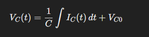
A capacitor is a two-terminal device that stores energy in the form of an electric field between its plates. Any time there are conductive plates separated by a dielectric (whether that be a material like fiberglass or even air), capacitance is formed. Their most important characteristic is their tendency to oppose change in voltage. Capacitors have a special time-dependent voltage-current relationship. The current through a capacitor depends on the rate of change of voltage:

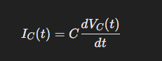
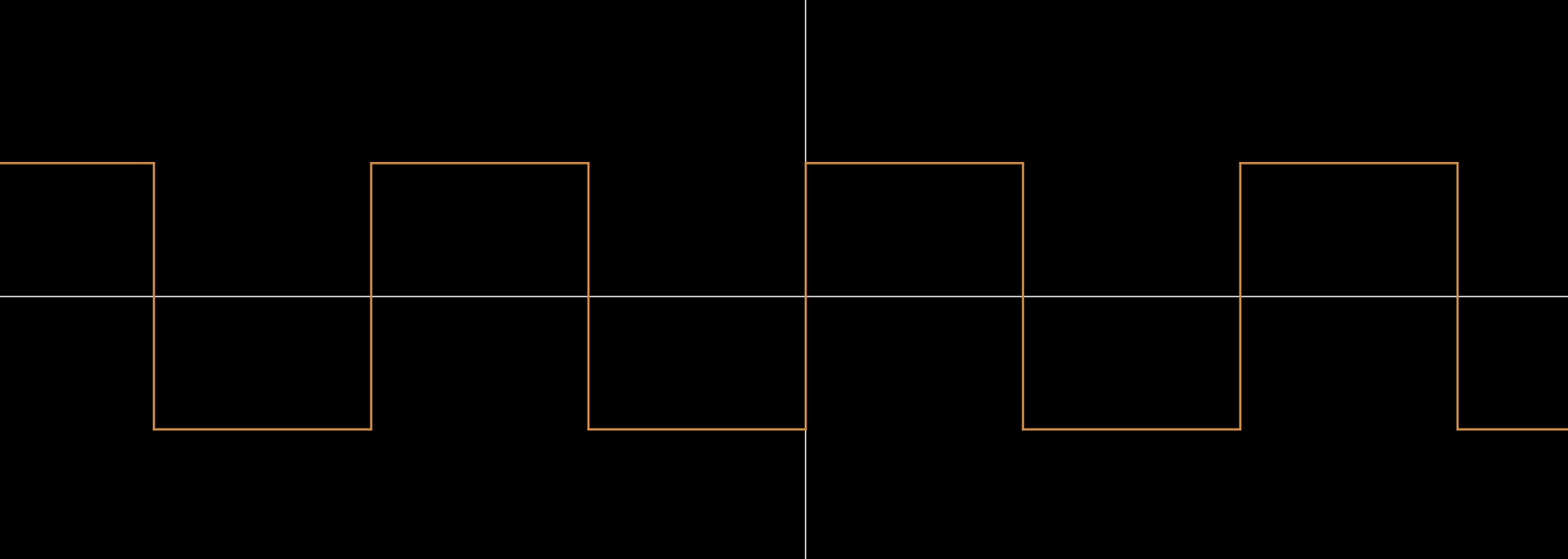
In an AC system, where voltage varies with time, a capacitor allows current to flow proportionally to the frequency of the signal. An important note is that to DC voltage (dV/dt = 0), a capacitor is essentially an open circuit. No current will flow through a capacitor connected to a DC voltage source.

Inductance: Opposition to Current Change

An inductor is a coil of wire that stores energy in the form of a magnetic field. It resists changes in the current flowing through it, which is opposite the role of the capacitor. Any time there is a conductor with current flowing through it, whether or not it is intentionally coiled, inductance is formed due to the resulting magnetic field. The voltage-current relationship is also time-dependent. Voltage across an inductor is proportional to the rate of change of current:

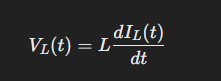
In an AC system, where current varies with time, the inductor produces a voltage that opposes this change. To DC current (dI/dT = 0), inductors act as a short circuit and no voltage is developed across them.

1.2 Reactance: Opposition to Alternating Current

What is reactance?

Reactance (denoted by X) is the frequency-dependent opposition that capacitors and inductors present to alternating current due to the energy stored in their magnetic or electric fields. It is the quantity that defines exactly how inductors and capacitors impact the phase relationship between voltage and current when they vary by time, and by how much they oppose change in current. Unlike resistance, which is constant, reactance varies with frequency.

Keep in mind that when discussing reactance, we are talking about opposition to change in current, not just opposition to current. This is why reactance varies with frequency.

Capacitive Reactance (Xc)

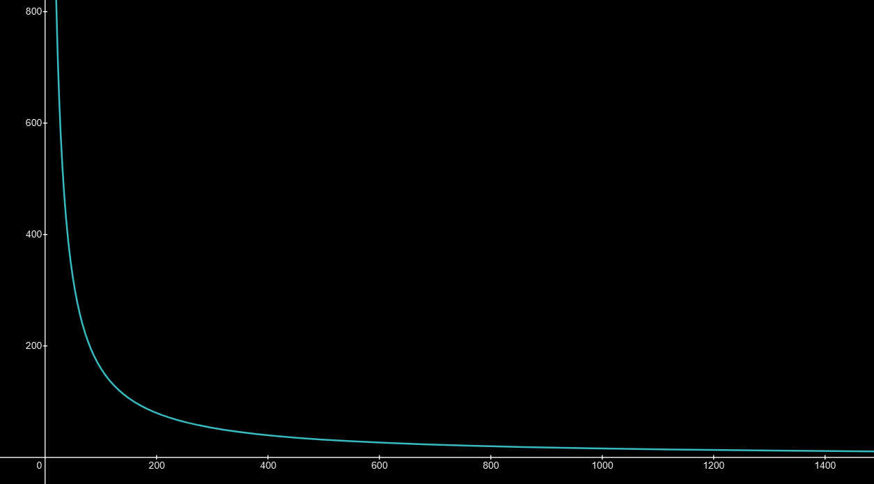
Capacitive reactance decreases with frequency. That is, the higher the frequency, the less capacitors oppose change in current. It is given by the following equation:

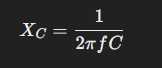
Looking back Equation 1, it is easy to see why capacitive reactance decreases with frequency. With increasing frequency, voltage varies more rapidly (dV/dt), leading to more of an allowance for current to flow through the capacitor.

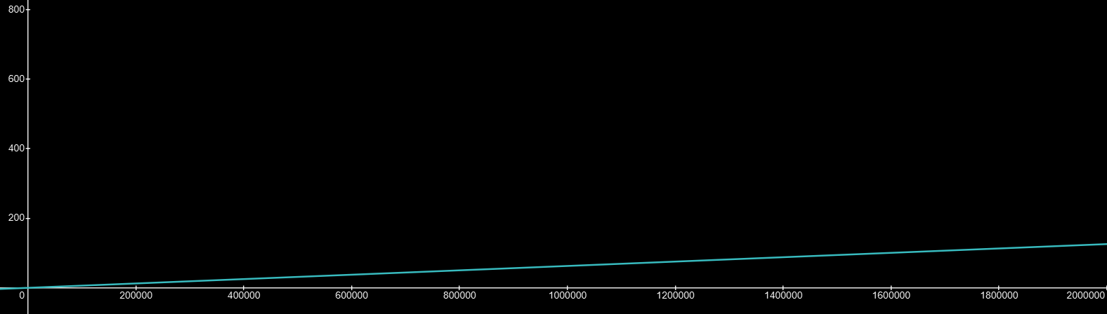
Inductive Reactance (Xl)

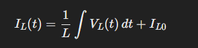
Inductive reactance has the opposite behavior of capacitive reactance. It increases with frequency, so the higher the frequency, the more it opposes change in current:

Equation 4 demonstrates this. The integral of a sinusoidal waveform at a given amplitude is always less than that of a constant signal at the same amplitude, so current decreases with frequency.

II. Impedance: Generalization of Resistance

In AC circuits, resistance alone does not fully describe the opposition to current flow. This is because capacitors and inductors introduce a dynamic, frequency-dependent element to this opposition, which is described by the concept of impedance. Impedance is the AC equivalent of resistance, but it is a more comprehensive quantity that accounts for both resistance and reactance. Because it includes reactance, its magnitude is frequency-dependent.

2.1 What is impedance?

Impedance (Z) describes the total opposition a circuit presents to a time-varying current due to resistance and energy storage in magnetic or electric fields. Unlike resistance, which is purely real, impedance is a complex quantity that includes a real component (resistance) and an imaginary component (reactance). When calculating the impedance of a circuit, the total reactance quantity is used:

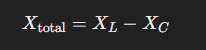
Since inductive and capacitive reactance have opposite effects on the circuit, they are subtracted algebraically (leading from lagging phase difference). This means that if a circuit is purely capacitive, its reactance is negative. The equation for total impedance is given by:

Reactance is imaginary because it represents the phase difference between voltage and current due to reactive elements, which do not dissipate energy, but store and release it cyclically. Thus, impedance has a phase angle (θ). The imaginary unit j is used to denote the 90-degree phase shift. By contrast, resistance, which dissipates energy as heat, is the real component, making impedance a complex quantity with both real and imaginary parts.

Complex numbers can be represented in both polar and rectangular coordinates because they inherently describe points or vectors in a 2D plane known as the complex plane. The rectangular representation aligns with standard Cartesian coordinate space, making it intuitive for addition and subtraction by treating the real and imaginary parts as independent components (resistance = x and reactance = y). On the other hand, polar coordinates better reflect the geometric nature of complex numbers and are useful to be treated as vectors for scaling and rotation. In polar form, impedance is given by:

The overall magnitude of impedance is given by:

2.2 Practical Implications of Impedance

Phase Relationships

Impedance governs the phase relationship between voltage and current in AC circuits:

• If X > 0 (inductive reactance dominates), current lags voltage
• If X < 0 (capacitive reactance dominates), current leads voltage

The phase angle is given by:

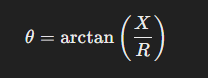
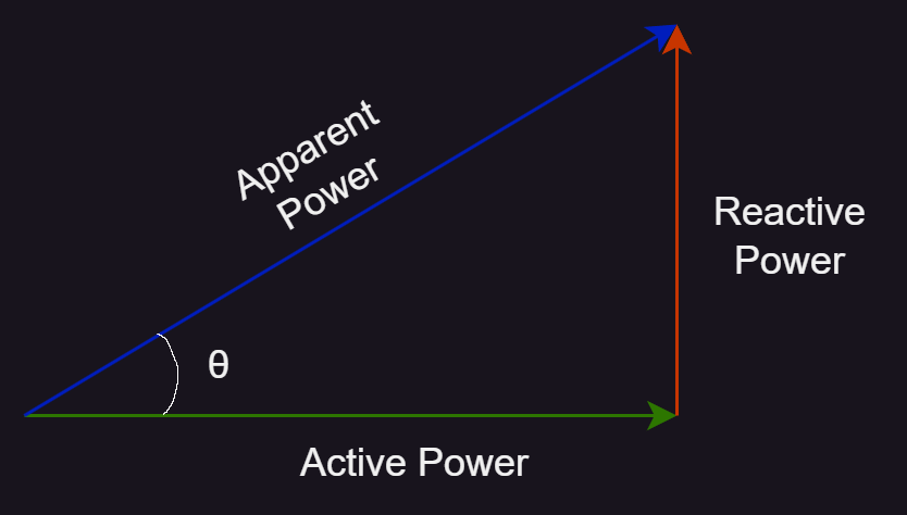
In most electronic circuits, particularly those involving power delivery or high-speed signals, a phase difference between voltage and current can lead to failures. For power delivery purposes, a non-zero phase angle means that some delivered power is wasted in reactive elements, alternating between source and load, and not actually able to be consumed by the load. This means that some power is wasted.

Power Delivery

Higher impedance, and thus larger phase angle, inhibits the ability of voltage regulators to supply current to the load. This leads to voltage spikes or sags manifested as noise. Recall Ohm's law, V = IZ. As the magnitude of Z increases for the same load current, voltage has to increase. A high Z at the load point can also form a voltage divider between parasitic inductance (impedance) in the current path and the load, which causes voltage sags. Both of these are harmful to electronics and must be minimized.

When current travels along a conductor to the load, it encounters parasitic impedance. For power delivery systems in a PCB, the conductor is often a flat, wide copper pour. In this case, the inductance is spreading inductance and dependent on the geometrical shape of the pour, not its size. If the load has any transient current demand, at any frequency, this inductance can contribute to power delivery system failure due to high impedance if something is not done to correct it. More inductance, and thus more reactance (recall Equation 6) means higher impedance, regardless of the frequency. To put these concepts into perspective:

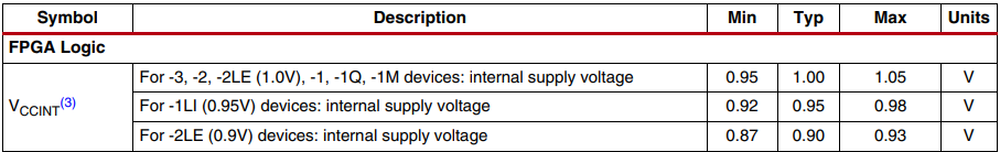
For the Artix-7 FPGA, a voltage sag or spike of only 50 mV is enough to shift out of the recommended operating conditions. This must be avoided at all costs, and impedance contributes to these spikes or sags.

III. Resonance in LC Circuits

When capacitive and inductive reactance cancel each other out (X = 0), the circuit is said to be operating at resonance. Resonance is one of the most intriguing concepts in AC circuit analysis and ties together all of the concepts discussed so far. It is often exploited for applications such as signal filtering, frequency selection, energy transfer, and decoupling. However, it can also potentially ruin a system's operation depending on the application.

3.1 What is Resonance?

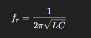
Resonance occurs at a specific frequency in an LC circuit when the inductive reactance (Xl) equals the capacitive reactance (Xc). At this frequency, known as the resonant frequency (fr), the effects of the inductor and capacitor cancel each other out, leaving the circuit with only its resistive impedance. The formula for calculating an LC circuit's resonant frequency is:

3.2 Series LC Resonance

In a series LC circuit, the inductor and capacitor are connected in series, and the total impedance is the sum of their reactances:

At resonance, Xl = Xc, so the total reactance is 0 (recall Equation 7). This means that the impedance is purely resistive with no reactance and no phase shift. At this frequency, the phase angle is zero. Current will follow voltage perfectly. The effect is that the circuit's impedance is minimized, allowing maximum current to flow (I = V / Z).

In a series LC configuration, the resonant frequency is the operating frequency at which maximum power can be transferred through it. This is essential for applications such as inductive cookers and some electromagnets. Since the impedance is minimal, series LC circuits at resonance are also widely used for decoupling purposes, to allow transient noise currents (or energy supply at that frequency) to flow as freely as possible through. This is one way of correcting the voltage sags or spikes due to parasitic inductance mentioned in Section 2.2.

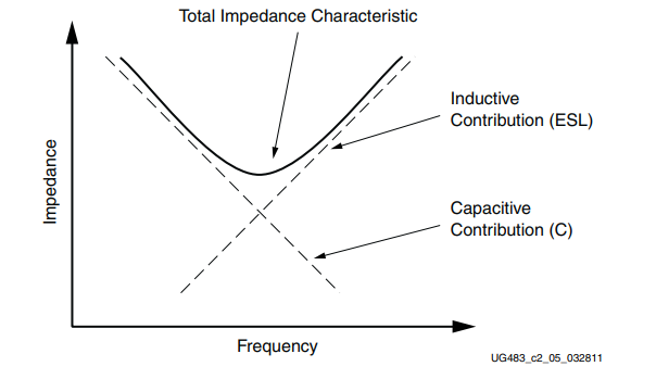
The resonant frequency marks the point at which the circuit transitions from functioning like a capacitor to being more inductive in nature. This is because the total impedance contains the vector sum of capacitive and inductive reactance; at lower frequencies, capacitive reactance is larger than inductive reactance, which dominates the circuit's behavior. At resonance, the circuit is purely resistive and is neither capacitive nor inductive. Above resonance, Xl becomes larger than Xc, so the total impedance is dominated by inductive reactance, making it behave like an inductor.

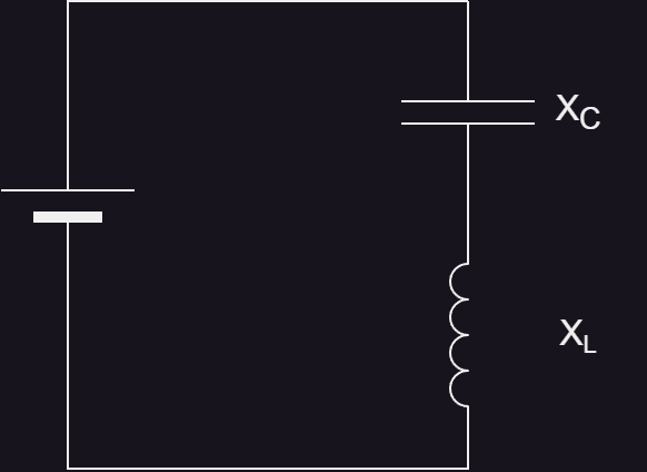
3.3 Parallel LC Resonance

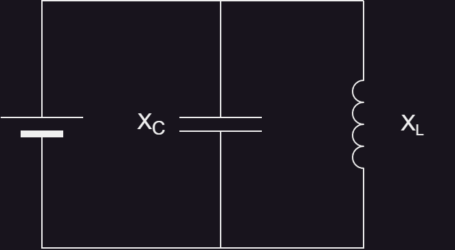
In a parallel LC circuit, the inductor and capacitor are connected in parallel, and the total impedance is determined by their reciprocal sum (the same as resistors in parallel):

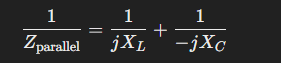
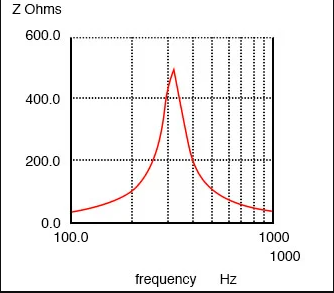
At resonance, Xl = Xc, so the reactances cancel each other out and, in an ideal circuit, impedance becomes infinite (Z becomes 0^-1, which implies 0 in the denominator, which approaches infinity). The effect is that the circuit blocks current at the resonant frequency.

A parallel LC circuit at resonance functions as a frequency rejector, attenuating signals at the resonant frequency while allowing others to pass. This can be beneficial for certain applications such as filters. However, for other applications, it is very problematic. For example, if a load (such as an FPGA or microprocessor) experiences a transient current demand at the resonant frequency of the parallel LC circuit formed by decoupling capacitors and parasitic power path inductance, the availability of energy to the load will be severely limited due to high impedance. This is called anti-resonance.

Below the resonant frequency, the capacitive reactance is larger, and the inductive reactance is smaller. So, the parallel LC circuit behaves more like an inductor below the resonant frequency because the low impedance of the inductor dominates over the high impedance of the capacitor in parallel (more current is flowing through the inductor than the capacitor). At the resonant point, the circuit entirely blocks current and is neither inductive nor capacitive. Above the resonant point, the lower impedance of the capacitor (due to lower capacitive reactance) dominates over the higher impedance of the inductor (due to higher inductive reactance), and the circuit behaves more like a capacitor.

3.4 Quality Factor and Bandwidth

Resonant LC circuits have a characteristic known as the quality factor (Q-factor). The Q-factor quantifies the sharpness of resonance. It is defined as:

Where bandwidth is the range of frequencies over which the circuit's impedance deviates significantly from its resonant value. A good way to think about Q-factor is as a parameter that can either flatten or sharpen the impedance characteristic curve (recall Figures 9 and 11).

A high Q-factor has a narrow bandwidth. This means that the resonance curve is sharper. The effect is that there is a very narrow range of frequency where the impedance is low (in series LC) or high (in parallel LC). You'd want this for applications such as precision filters and oscillators, but for other applications (such as decoupling networks), you want a higher bandwidth for effective operation over a wide range of frequencies.

A low Q-factor has a wide bandwidth. This means that the resonance curve is flatter, meaning there is a wider range of low or high impedance for the circuit. This is used in applications requiring broader frequency response.

Q-factor is inversely proportional to resistance: as resistance increases, Q-factor decreases. So, to get a wider bandwidth (meaning low Q-factor), you'd want to add series resistance as a damper.

Conclusion

AC circuit analysis is a cornerstone of electronics engineering, providing the tools to understand and design systems that rely on dynamic, time-varying signals (or those which have unintentional time-varying signals). These principles are the backbone of countless applications, from filtering signals to optimizing power delivery. There is much more to cover that is outside the scope of this post (or too technical), but this is a good starting point.

This knowledge provides a solid foundation for practical applications. In the coming posts, we'll explore how these concepts apply to controlling inductive loads intelligently. We'll also look at how power distribution systems for devices like FPGAs and microprocessors rely on AC circuit analysis topics despite operating in a DC environment. Understanding the topics in this article is crucial to doing good design work, regardless of the application.